SeaSenseLib Demo

This notebook demonstrates the capabilities of SeaSenseLib for reading oceanographic instrument data from various formats, writing it to netCDF and making basic plots or statistical calculations.

Overview

SeaSenseLib is a Python library for reading, converting, and plotting oceanographic sensor data from various instrument formats. It provides:

Simple API with ssl.read() and ssl.write() functions
Readers for multiple formats (CNV, NetCDF, RBR, ADCP, etc.)
Writers for data export (NetCDF, CSV, Excel)
Plotters for oceanographic visualizations via ssl.plot.*
Processors for basic statistical calculations or data manipulation

Generalised API features

The SeaSenseLib API simplifies common tasks:

import seasenselib as ssl

# Read any supported format into an xarray dataset
data = ssl.read('sensor_data.cnv')

# Create oceanographic plots
ssl.plot('depth-profile', profile_data, title="CTD Profile")
ssl.plot('ts-diagram', profile_data, title="T-S Diagram")
ssl.plot('time-series', profile_data, parameters=['temperature'], title="CTD Profile T-S Diagram")

# Export to various formats
ssl.write(data, 'output.nc')   # NetCDF
ssl.write(data, 'output.csv')  # CSV

[1]:

import numpy as np
import matplotlib.pyplot as plt
import warnings
warnings.filterwarnings('ignore')  # Suppress warnings for cleaner output

# Import SeaSenseLib
import seasenselib as ssl

# For processors, we directly import each processor
from seasenselib.processors import SubsetProcessor, StatisticsProcessor

# Set up matplotlib for inline plotting
plt.style.use('seaborn-v0_8')
plt.rcParams['figure.figsize'] = (10, 6)

print("✓ SeaSenseLib demo environment ready!")
print(f"✓ SeaSenseLib version: {ssl.__version__}")

✓ SeaSenseLib demo environment ready!
✓ SeaSenseLib version: 0.3.0

1. Reading Data from Different Formats

SeaSenseLib can read data from various oceanographic instruments. Let’s start with the example data files.

1.1 Reading CTD Profile Data (CNV Format)

First, let’s read a vertical CTD profile from a SeaBird CNV file. SeaSenseLib uses the python package pycnv to handle Seabird files, then returns data in an xarray dataset.

Note: The pycnv package is installed automatically as a dependency when you install SeaSenseLib via pip. You do not need to install it separately.

[2]:

# Read CTD profile data using `ssl.read()`
profile_data = ssl.read("../examples/MSM121_054_1db.cnv") # Alternative: sea-practical-2023.cnv

print("CTD Profile Dataset:")
print(f"Dimensions: {dict(profile_data.dims)}")
print(f"Data variables: {list(profile_data.data_vars)}")
print(f"Coordinates: {list(profile_data.coords)}")
print(f"\nData shape: {profile_data.sizes}")

type(profile_data)

INFO:pycnv: Opening file: ../examples/MSM121_054_1db.cnv
WARNING:pycnv:Could not compute datetime dates based on timeM
INFO:pycnv:Dates computed based on timeS

Date
Computing date
CTD Profile Dataset:
Dimensions: {'time': 3593}
Data variables: ['conductivity_1', 'conductivity_2', 'flag', 'oxygen_1', 'oxygen_2', 'pressure', 'salinity', 'temperature_1', 'temperature_2', 'timeQ', 'timeS', 'depth', 'density', 'potential_temperature']
Coordinates: ['latitude', 'longitude', 'time']

Data shape: Frozen({'time': 3593})

[2]:

xarray.core.dataset.Dataset

1.2 Reading Time Series Data (Moored Instrument)

Now let’s read time series data from a moored instrument, again from Seabird in native *.cnv format.

[3]:

# Read time series data from moored microCAT time series
timeseries_data = ssl.read("../examples/denmark-strait-ds-m1-17.cnv")

print("Time Series Dataset:")
print(f"Dimensions: {dict(timeseries_data.dims)}")
print(f"Data variables: {list(timeseries_data.data_vars)}")
print(f"Time range: {timeseries_data.time.min().values} to {timeseries_data.time.max().values}")
print(f"Duration: {len(timeseries_data.time)} measurements")

INFO:pycnv: Opening file: ../examples/denmark-strait-ds-m1-17.cnv
WARNING:pycnv:Could not compute datetime dates based on timeM
WARNING:pycnv:Could not compute datetime dates based on timeS
INFO:pycnv:Dates computed based on start_date and time_interval

Date
Computing date
Time Series Dataset:
Dimensions: {'time': 59088}
Data variables: ['conductivity', 'flag', 'pressure', 'salinity', 'scan', 'temperature', 'timeJ', 'depth', 'density', 'potential_temperature']
Time range: 2017-09-12T09:40:29.000000000 to 2017-09-19T05:48:19.000000000
Duration: 59088 measurements

3. Data Conversion and Export

SeaSenseLib can export data to various formats while preserving metadata and following CF conventions. Note that if the demo output file already exists, ssl will not overwrite it.

[6]:

# Convert CNV to NetCDF and CSV using the new API
ssl.write(profile_data, 'demo_output_profile.nc')
print("✓ Exported to NetCDF: demo_output_profile.nc")

ssl.write(profile_data, 'demo_output_profile.csv')
print("✓ Exported to CSV: demo_output_profile.csv")

✓ Exported to NetCDF: demo_output_profile.nc
✓ Exported to CSV: demo_output_profile.csv

3.1 Verify NetCDF Export

Let’s read back the NetCDF file to verify the export worked correctly:

[7]:

# Read back the exported NetCDF file using the new API
netcdf_data = ssl.read('demo_output_profile.nc')

print("Exported NetCDF file structure:")
print(f"Dimensions: {dict(netcdf_data.dims)}")
print(f"Variables: {list(netcdf_data.data_vars)}")
print(f"Data preserved: {len(netcdf_data.data_vars)} variables exported successfully")
print("\n✓ NetCDF export/import successful!")

Exported NetCDF file structure:
Dimensions: {'time': 3593}
Variables: ['conductivity_1', 'conductivity_2', 'flag', 'oxygen_1', 'oxygen_2', 'pressure', 'salinity', 'temperature_1', 'temperature_2', 'timeQ', 'timeS', 'depth', 'density', 'potential_temperature']
Data preserved: 14 variables exported successfully

✓ NetCDF export/import successful!

4. Data Visualization

SeaSenseLib provides a few plotting tools for oceanographic data visualization:

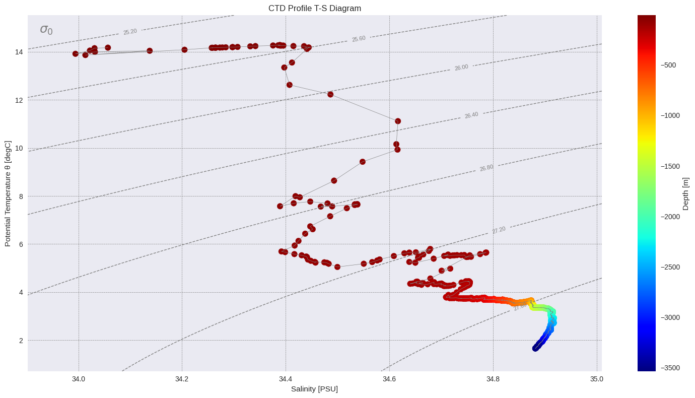
4.1 Temperature-Salinity (T-S) Diagram

T-S diagrams show the relationship between temperature and salinity with density isolines.

Note: The plotting tool by default expects variables temperature and salinity which are set in parameters.py. If you’re working with CTD data, and you want to specify to always use temperature_1, then this can be updated in parameters.py. For the purpose of this demonstration, we’ll create new variable temperature.

[8]:

# Add variable 'temperature'
profile_data['temperature'] = profile_data['temperature_1']

ssl.plot('ts-diagram', profile_data, title="CTD Profile T-S Diagram")
print("✓ T-S diagram created")

✓ T-S diagram created

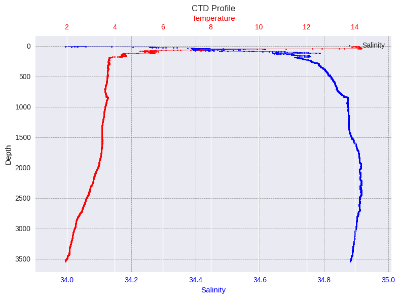
4.2 Vertical Profile Plot

Display the CTD cast as a vertical profile showing how parameters change with depth:

[9]:

# Create vertical profile plot using the new API
ssl.plot('depth-profile', profile_data, title="CTD Profile")
print("✓ Vertical profile plot created")

✓ Vertical profile plot created

4.3 Time Series Plots

For the moored instrument data, let’s create time series plots:

[10]:

ssl.plot('time-series', timeseries_data, parameters=['temperature'], title="Temperature Time Series")
print("✓ Temperature time series created")

✓ Temperature time series created

[11]:

# Multi-parameter time series
# You can plot multiple parameters at once, but this plotter uses the same y-axis limits for all parameters.
available_ts_params = [p for p in ['temperature', 'salinity', 'pressure'] if p in timeseries_data.data_vars]

if len(available_ts_params) >= 2:
    ssl.plot('time-series', timeseries_data, parameters=available_ts_params, title="CTD Profile T-S Diagram")
    print(f"✓ Multi-parameter time series created for: {available_ts_params[:2]}")
else:
    print(f"Insufficient parameters for multi-plot. Available: {available_ts_params}")

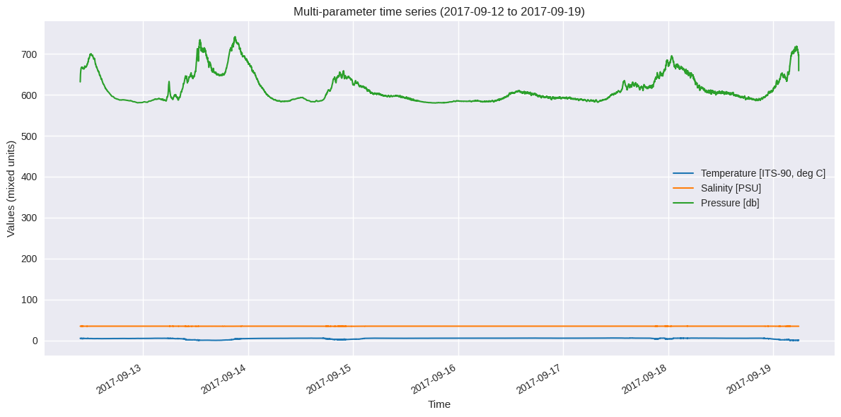
✓ Multi-parameter time series created for: ['temperature', 'salinity']

5. Further data tools

SeaSenseLib provides basic tools for subsetting and statistics:

5.1 Data Subsetting

Extract specific depth ranges or time periods:

[12]:

# Subset profile data by depth (if pressure/depth data available)
subset_processor = SubsetProcessor(profile_data)

if 'pressure' in profile_data.data_vars:
    # Subset to upper 50 dbar (approximately 50 meters)
    shallow_data = subset_processor.set_parameter_name('pressure').set_parameter_value_min(0).set_parameter_value_max(50).get_subset()
    print(f"Original data points: {len(profile_data.pressure)}")
    print(f"Shallow subset (0-50 dbar): {len(shallow_data.pressure)}")
    print(f"Pressure range in subset: {shallow_data.pressure.min().values:.1f} - {shallow_data.pressure.max().values:.1f} dbar")
else:
    print("Pressure data not available for depth subsetting")

Original data points: 3593
Shallow subset (0-50 dbar): 44
Pressure range in subset: 7.0 - 50.0 dbar

[13]:

import pandas as pd
# Subset time series data by time period
if 'time' in timeseries_data.coords and len(timeseries_data.time) > 100:
    ts_subset_processor = SubsetProcessor(timeseries_data)
    # Get the first half of the time series
    start_time = timeseries_data.time.min()
    mid_time = timeseries_data.time[len(timeseries_data.time)//2]

    first_half = ts_subset_processor.set_time_min(pd.Timestamp(start_time.values)).set_time_max(pd.Timestamp(mid_time.values)).get_subset()

    print(f"Original time series length: {len(timeseries_data.time)}")
    print(f"First half subset length: {len(first_half.time)}")
    print(f"Time range in subset: {first_half.time.min().values} to {first_half.time.max().values}")
else:
    print("Time data not suitable for subsetting")

Original time series length: 59088
First half subset length: 29545
Time range in subset: 2017-09-12T09:40:29.000000000 to 2017-09-15T19:44:29.000000000

5.2 Statistical Analysis

Calculate statistics for the datasets:

[14]:

# Compare statistics between full profile and shallow subset
if 'pressure' in profile_data.data_vars and 'temperature' in profile_data.data_vars:
    full_temp_processor = StatisticsProcessor(profile_data, 'temperature')
    full_stats = full_temp_processor.get_all_statistics()

    shallow_temp_processor = StatisticsProcessor(shallow_data, 'temperature')
    shallow_stats = shallow_temp_processor.get_all_statistics()

    print("=== Temperature Statistics Comparison ===")
    print(f"Full profile - Mean: {full_stats['mean']:.3f}°C, Range: {full_stats['min']:.3f} - {full_stats['max']:.3f}°C")
    print(f"Shallow (0-50m) - Mean: {shallow_stats['mean']:.3f}°C, Range: {shallow_stats['min']:.3f} - {shallow_stats['max']:.3f}°C")

    temp_diff = shallow_stats['mean'] - full_stats['mean']
    print(f"\nTemperature difference (shallow - full): {temp_diff:.3f}°C")
    if temp_diff > 0:
        print("→ Shallow waters are warmer (typical thermocline pattern)")
    else:
        print("→ Shallow waters are cooler")

=== Temperature Statistics Comparison ===
Full profile - Mean: 3.318°C, Range: 1.944 - 14.286°C
Shallow (0-50m) - Mean: 13.701°C, Range: 9.430 - 14.286°C

Temperature difference (shallow - full): 10.382°C
→ Shallow waters are warmer (typical thermocline pattern)

Next Steps

To learn more about SeaSenseLib:

Documentation: Check the full documentation for detailed API reference
CLI Usage: Try the command-line interface with seasenselib --help
More Formats: Explore support for RBR, ADCP, and other instrument formats (see the Moored Instruments demo)
Custom Processing: Implement custom readers and processors for your specific needs
Integration: Integrate SeaSenseLib into your oceanographic data processing workflows

Example CLI Commands

# List supported formats
seasenselib formats

# Convert CNV to NetCDF
seasenselib convert -i examples/sea-practical-2023.cnv -o output.nc

# Create plots
seasenselib plot ts-diagram -i output.nc -o ts_diagram.png
seasenselib plot depth-profile -i output.nc -o profile.png
seasenselib plot time-series -i examples/denmark-strait-ds-m1-17.cnv -p temperature

Happy oceanographic data processing! 🌊