OceanArray processing framework
This document outlines the stages of processing for data from moored instruments. Processing is separated into “instrument-level” processing (actions performed on a single instrument for a single deployment), “mooring-level” processing (actions performed on a mooring consisting of instruments deployed at the same x/y location), and “array-level” processing (actions performed on multiple moorings used together).
Initial examples are built from the RAPID project, which is a well-established mooring array in the Atlantic Ocean, which uses an array of moored instruments to measure the Atlantic Meridional Overturning Circulation (AMOC).
Principles:
Modular: Each stage has clearly defined inputs and outputs.
Adaptable: While RAPID and similar projects guide the structure, this framework supports different instrument types, platforms, and processing strategies.
Reproducible: Every transformation step should be traceable, with logs, versioning, and metadata.
Incremental: Intermediate outputs should be storable and reloadable for downstream processing.
Final datasets are stored in a common format (CF-netCDF following OceanSITES) with consistent metadata for analysis or transport diagnostics.
Instrument-level processing
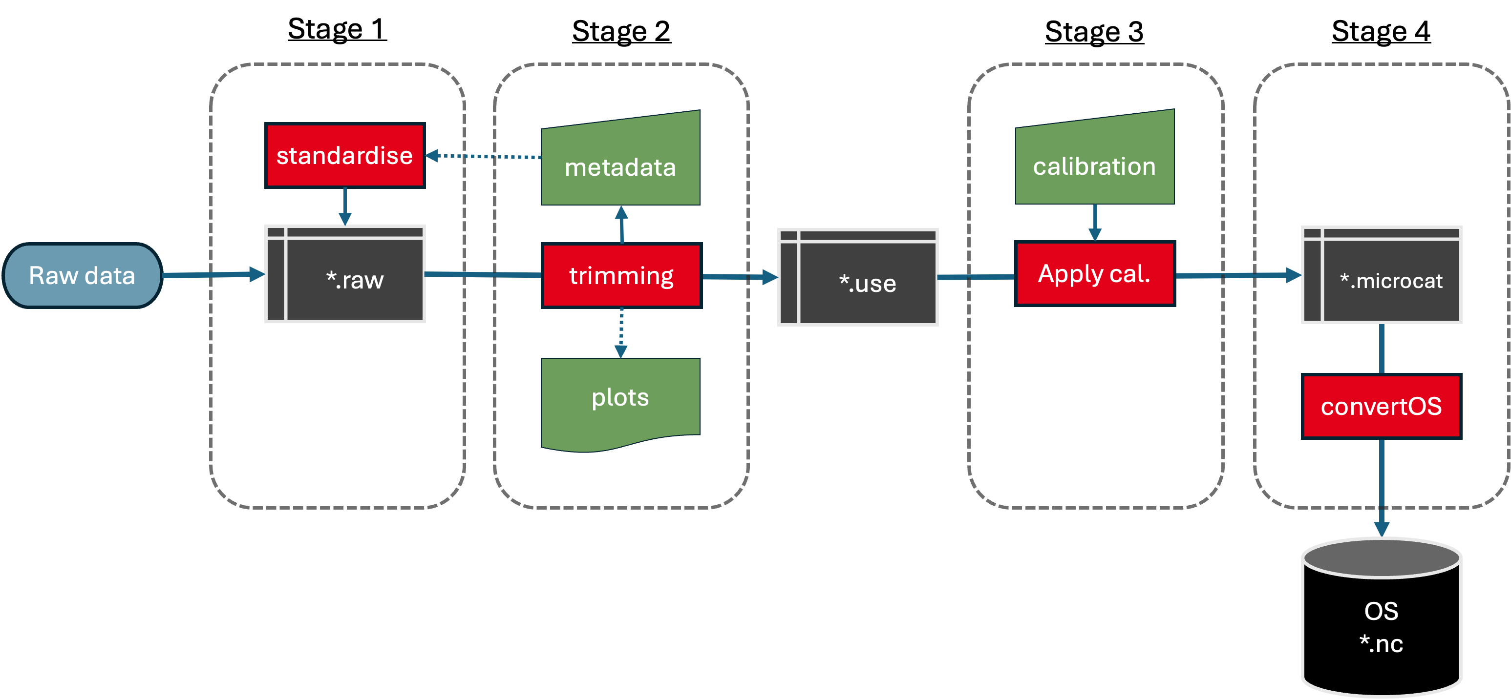
Instrument-level processing workflow.
The instrument-level processing carries out 2 main steps:
Stage 0: Downloading raw instrument files (e.g., .cnv, .asc).
Stage 1: Converting data files to a consistent (internal) format.
Stage 2: Trimming the record to the deployment period (i.e., removing the launch and recovery periods) and applying clock corrections.
Stage 3: Applying automatic QC, i.e. global range tests and spike tests from ioos_qc QARTOD.
Stage 3.5: Apply calibrations to the moored instrument and create a traceable log of the calibration process.
Stage 4: Convert data to a common format for onward use with rich metadata.
The first step step is downloading data from instruments. This is typically using manufacturers’ software and some of the downloaded files may be in proprietary formats (e.g., SeaBird .cnv format). Formats can also change over time or depending on settings used when downloading the data, hence the need for the “standardisation” step. Stage 0 is typically performed at sea as soon as a mooring is recovered and instruments are available.
Note
Stage 2 clock corrections are only necessary if the clock on the instrument was set up incorrectly (normally should be UTC to the nearest second) or if the instrument drifts over the deployment period (usually small/negligible for microCATs, i.e. a clock drift of a few seconds or up to a minute is usually ignored except for bottom pressure sensors).
Note
Stage 3 only involves applying calibration corrections. The corrections should be determined in a separate step, e.g., by comparing the instrument data with the CTD during a calibration cast (pre- and post-deployment) or with laboratory calibrations (pre- and/or post-deployment).
RAPID Analogy
Stage 0: Download raw instrument files (e.g., .cnv, .asc). The initial conversion to the RDB (or RODB) format is called “stage 1” and takes place while still onboard the ship. Stage 2 is mainly trimming to the deployment period, which requires some minor iteration between running the processing, updating the mooring-level metadata (contained in a RAPID *info.dat file), and then re-running the processing. Outputs are the *.use RDB format file. The third stage is performed after the cruise, and isn’t necessarily referred to by the RAPID project as “stage 3”. This is done also with some iterative steps where corrections are applied making various choices (linear change between pre- and post-cruise calibrations) or using only the pre- or post-cruise cal dip, and making different versions of the *.microcat file in RDB format. Each variation of the processing also produces a parallel *.microcat.txt file recording the choices made. A final choice may be made only after comparing to auxiliary data or other instruments on the mooring, so while this falls within “instrument-level” processing because it’s performed on a single instrument, the inputs may be broader.
Further details:
Data Acquisition (Download in proprietary formats) describes downloading raw instrument files.
1. Standardisation (Internally-consistent format) describes how to convert the raw instrument files to an internally-consistent format (e.g., RBD or netCDF).
2. Trimming to Deployed period describes how to trim the data to the deployment period and apply clock corrections.
3. Automatic QC flagging describes the approach for automatically generating and adding quality control flags to the data parameters (geophysical ones, e.g., TEMP, CNDC, PRES).
3. Calibration (Instrument-level Corrections) describes how to apply calibration corrections to the instrument data and create a traceable log of the calibration process.
4. Conversion to OS format describes how to convert the data to a common format (e.g., CF-netCDF) with rich metadata.
Mooring-level processing
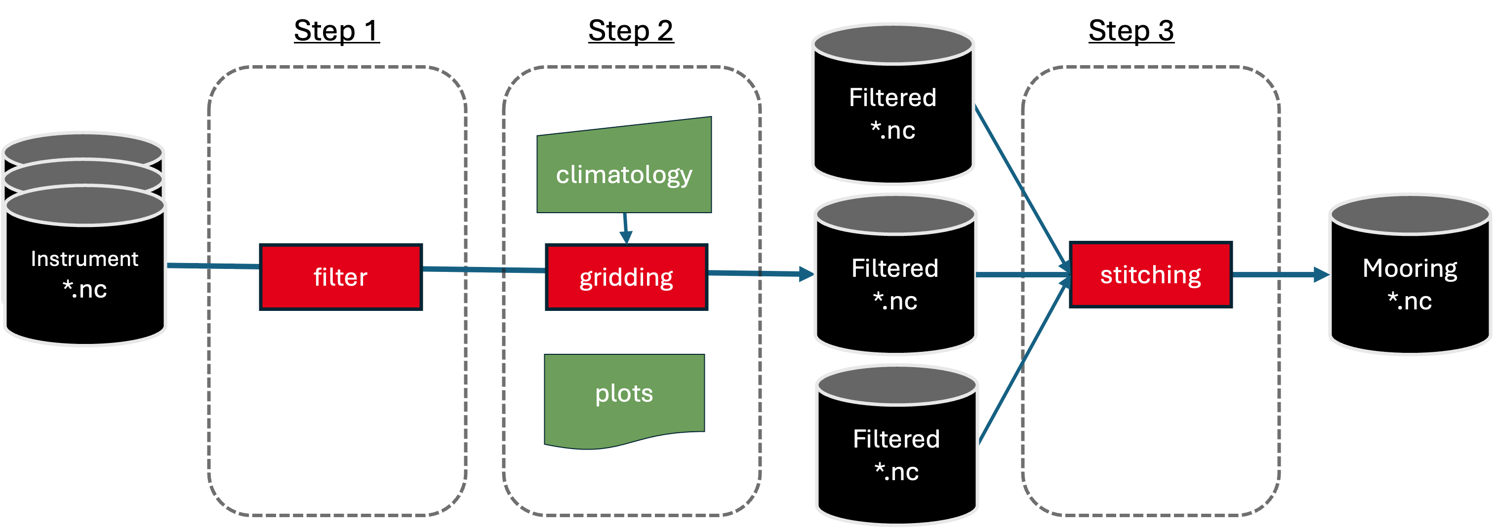
Mooring-level processing workflow.
The previous steps (stage 0 to stage 3) are applied per instrument, per deployment. When multiple instruments are deployed on the same tall mooring, the next steps can be applied to produce a vertical profile of data.
Step 1: Time gridding onto a consistent time axis for all instruments on a mooring. Low-pass filtering or other de-tiding procedures can also be applied.
Step 2: Vertical gridding onto a standard pressure grid, combining measurements from multiple instruments on the same mooring
Step 3: Concatenating (in time) the data from multiple mooring deployments at a single x/y location.
Outputs can be stored in updated OceanSites format file(s) which include details of processing steps in the metadata.
Note
Step 1 may include filtering to remove tides, and subsampling to a coarser grid for data decimation, depending on the scientific aims of the project.
Note
Step 2 as included here assumes that all individual instruments have a pressure sensor and so they know their vertical position. If this is not the case, then a “virtual” pressure record may need to be created, e.g. by interpolating between two sensors with pressure measurements.
RAPID Analogy
For RAPID, data are de-tided by using a 2-day, 6th order Butterworth low-pass filter. Data are then subsampled to 12 hour intervals for onward processing. Vertical gridding is done by using climatological (monthly) profiles of temperature and salinity built from hydrographic (CTD and Argo profile) data. Concatenating in time is done with a simple application of interp1.m in Matlab onto a uniform 12-hourly time axis.
Further details:
Step 1: Time Gridding and Optional Filtering describes how to apply a low-pass filter and subsample the time series to a common time axis.
Step 2: Vertical Gridding describes how to vertically interpolate the data onto a standard pressure grid.
Concatenate Deployments describes how to concatenate multiple deployments at a single x/y location into a continuous time series.
Array-level processing
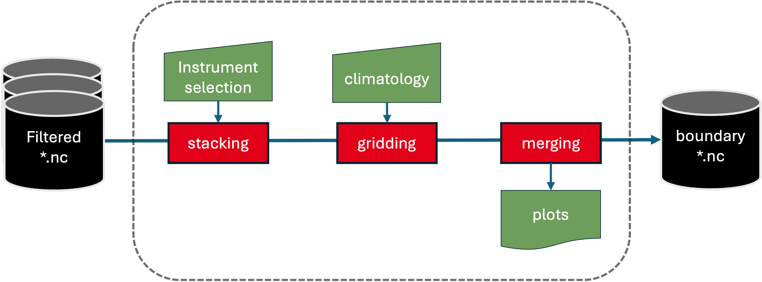
Array-level processing workflow.
For boundary profiles, this step starts from the time-gridded individual instrument records produced in the previous steps, stacking them and sorting them vertically at east time step, and then re-doing the vertical regridding now across instrument data from multiple moorings. This helps minimize data gaps and ensures smooth transitions across deployments. Note that this may not have any method to flag or identify possibly statically unstable profiles.
RAPID Analogy
For RAPID, this is done by merging the mooring sites WB2, WB3, and WBH2 where data from 0-3800 dbar are used from WB2, then the next deeper instruments from WBH2 and then WB3 are added. These sites, deployed across a sloping ocean boundary, improve coverage along the boundary (e.g., when WB2 ends at 3800 dbar, and WB3 at 4500 dbar). The final output is a merged “West” profile, ready for use in transport calculations.
Further details:
Multi-site Merging describes how to merge multiple mooring sites into a single boundary profile.
Further Analysis
The notes below are a stub.
Transbasin Transport
Description: TEOS-10 conversion, dynamic height, and shear.
Actions:
Convert to Absolute Salinity and Conservative Temp.
Compute dynamic height and geostrophic shear.
Inputs: T/S/P profiles
Choices: reference pressure
Outputs: Dynamic height fields
RAPID Analogy: gsw_geo_strf_dyn_height
Velocity-Based Transports
Description: Processing of WBW/ADCP data.
Actions:
Filter, vertically/horizontally interpolate.
Sum over depth × width.
Inputs: Velocity data + bathymetry
Outputs: WBW transport fields
RAPID Analogy: WBW/Johns et al. 2008
Composite Transport and Mass Compensation
Description: Combine transports and ensure mass balance.
Actions:
Combine all components.
Hypsometric compensation.
Cumulative transports.
Inputs: Component transports + bathymetry
Outputs: td_total, streamfunction
RAPID Analogy: transports.m, stream2moc.m
MOC Time Series and Diagnostics
Description: Final diagnostics and time series generation.
Actions:
Compute overturning strength and depth.
Integrate layer transports (e.g. thermocline, NADW).
Apply final time filtering.
Outputs: MOC time series, diagnostics, plots
Summary Table
Step |
Name |
Description |
RAPID Equivalent |
|---|---|---|---|
0 |
Acquisition |
Download raw instrument files (e.g., .cnv, .asc) |
Stage 0 |
1 |
Standardisation |
Convert raw files to CF-netCDF with metadata |
Stage 1 (RDB conversion) |
2 |
Trimming & QC |
Restrict to deployment period, apply initial QC |
Stage 2 (*.use) |
3 |
Calibration |
Apply CTD/lab-based corrections (salinity, pressure) |
Post-cruise |
A |
Time Filtering |
Remove tides, subsample time series |
auto_filt |
B |
Vertical Gridding |
Interpolate onto standard pressure grid |
hydro_grid, con_tprof0 |
C |
Concatenation |
Join deployments into continuous mooring records |
Internal |
D |
Boundary Merging |
Merge multiple moorings (e.g., WB2–WB4) into slope profile |
West, East, Marwest merged profiles |